What happens to a product with elastic demand when the the price of that item increases?

Sensitivity of quantity to toll

A good'southward price elasticity of demand ( ${\displaystyle E_{d}}$ , PED) is a measure of how sensitive the quantity demanded is to its price. When the price rises, quantity demanded falls for almost whatsoever good, but information technology falls more than for some than for others. The price elasticity gives the pct change in quantity demanded when in that location is a one percent increment in price, holding everything else abiding. If the elasticity is −ii, that means a 1 per centum price rise leads to a two percent decline in quantity demanded. Other elasticities measure how the quantity demanded changes with other variables (e.yard. the income elasticity of need for consumer income changes).^[1]

Price elasticities are negative except in special cases. If a proficient is said to have an elasticity of ii, it almost always means that the skilful has an elasticity of −2 according to the formal definition. The phrase "more than rubberband" means that a good's elasticity has greater magnitude, ignoring the sign. Veblen and Giffen goods are 2 classes of goods which have positive elasticity, rare exceptions to the law of demand. Demand for a adept is said to be inelastic when the elasticity is less than ane in absolute value: that is, changes in price accept a relatively small-scale issue on the quantity demanded. Demand for a skillful is said to be elastic when the elasticity is greater than 1. A good with an elasticity of −two has rubberband demand because quantity falls twice equally much as the cost increase; an elasticity of -0.5 has inelastic demand because the quantity response is half the price increase.^[ii]

Acquirement is maximised when price is set so that the elasticity is exactly one. The good's elasticity can be used to predict the incidence (or "burden") of a tax on that expert. Various research methods are used to determine price elasticity, including examination markets, assay of historical sales information and conjoint analysis.

Definition [edit]

The variation in need in response to a variation in toll is called price elasticity of demand. It may also be defined equally the ratio of the pct change in quantity demanded to the percentage change in cost of particular commodity.^[3] The formula for the coefficient of toll elasticity of demand for a good is:^{[4] [five] [vi]}

${\displaystyle E_{\langle p\rangle }={\frac {\Delta Q/Q}{\Delta P/P}}}$

where ${\displaystyle P}$ is the price of the good demanded, ${\displaystyle \Delta P}$ is how much it changed, ${\displaystyle Q}$ is the quantity of the skilful demanded, and ${\displaystyle \Delta Q}$ is how much it changed. In other words, we tin say that the price elasticity of demand is the pct change in demand for a article due to a given pct alter in the price. If the quantity demanded falls 20 tons from an initial 200 tons after the cost rises $5 from an initial price of $100, so the quantity demanded has fallen 10% and the cost has risen v%, so the elasticity is (−10%)/(+5%) = −2.

The price elasticity of demand is ordinarily negative because quantity demanded falls when price rises, as described by the "law of demand".^[5] 2 rare classes of appurtenances which have elasticity greater than 0 (consumers purchase more if the price is college) are Veblen and Giffen goods.^[7] Since the price elasticity of demand is negative for the vast majority of goods and services (dissimilar well-nigh other elasticities, which take both positive and negative values depending on the good), economists often leave off the word "negative" or the minus sign and refer to the price elasticity of demand equally a positive value (i.e., in absolute value terms).^[6] They will say "Yachts have an elasticity of ii" meaning the elasticity is −two. This is a mutual source of confusion for students.

Depending on its elasticity, a adept is said to have elastic demand (> i), inelastic demand (< 1), or unitary elastic demand (= 1). If need is elastic, the quantity demanded is very sensitive to toll, e.g. when a ane% rise in price generates a 10% decrease in quantity. If demand is inelastic, the good'south need is relatively insensitive to price, with quantity changing less than toll. If demand is unitary rubberband, the quantity falls past exactly the percentage that the price rises. Two important special cases are perfectly elastic demand (= ∞), where even a small-scale rise in price reduces the quantity demanded to nada; and perfectly inelastic demand (= 0), where a rise in price leaves the quantity unchanged. The to a higher place measure of elasticity is sometimes referred to as the own-price elasticity of demand for a expert, i.e., the elasticity of need with respect to the skillful's ain price, in lodge to distinguish it from the elasticity of demand for that good with respect to the change in the price of some other good, i.e., an independent, complementary, or substitute adept.^[3] That two-good type of elasticity is called a cross-toll elasticity of demand.^{[8] [9]} If a 1% rise in the price of gasoline causes a 0.5% fall in the quantity of cars demanded, the cantankerous-price elasticity is ${\displaystyle E_{cg}^{d}=(-0.5\%)/(+1\%)=-0.5.}$

Every bit the size of the price alter gets bigger, the elasticity definition becomes less reliable for a combination of 2 reasons. Commencement, a good'southward elasticity is not necessarily constant; information technology varies at dissimilar points along the demand bend considering a one% alter in cost has a quantity effect that may depend on whether the initial price is high or low.^{[10] [11]} Contrary to common misconception, the price elasticity is non constant even along a linear need bend, but rather varies along the curve.^[12] A linear demand bend's slope is constant, to be certain, only the elasticity tin can change even if ${\displaystyle \Delta P/\Delta Q}$ is constant.^{[xiii] [14]} There does be a nonlinear shape of demand curve forth which the elasticity is constant: ${\displaystyle P=aQ^{1/E}}$ , where ${\displaystyle a}$ is a shift constant and ${\displaystyle Due east}$ is the elasticity.

Second, percentage changes are not symmetric; instead, the percentage modify between any two values depends on which one is chosen as the starting value and which as the ending value. For instance, suppose that when the price rises from $10 to $16, the quantity falls from 100 units to lxxx. This is a toll increase of sixty% and a quantity decline of twenty%, an elasticity of ${\displaystyle (-20\%)/(+60\%)\approx -0.33}$ for that office of the demand curve. If the price falls from $xvi to $10 and the quantity rises from 80 units to 100, all the same, the price decline is 37.v% and the quantity proceeds is 25%, an elasticity of ${\displaystyle (+25\%)/(-37.five\%)=-0.67}$ for the same part of the curve. This is an example of the alphabetize number problem.^{[15] [16]}

Ii refinements of the definition of elasticity are used to deal with these shortcomings of the bones elasticity formula: arc elasticity and bespeak elasticity.

Arc elasticity [edit]

Arc elasticity was introduced very early on past Hugh Dalton. It is very similar to an ordinary elasticity problem, but it adds in the index number problem. Arc Elasticity is a second solution to the asymmetry trouble of having an elasticity dependent on which of the two given points on a demand curve is chosen every bit the "original" point will and which as the "new" one is to compute the per centum change in P and Q relative to the average of the two prices and the boilerplate of the two quantities, rather than merely the change relative to i point or the other. Loosely speaking, this gives an "average" elasticity for the section of the actual need bend—i.e., the arc of the curve—between the two points. Equally a result, this mensurate is known every bit the arc elasticity, in this case with respect to the price of the good. The arc elasticity is divers mathematically as:^{[16] [17] [18]}

${\displaystyle E_{d}={\frac {\frac {P_{i}+P_{two}}{2}}{\frac {Q_{d_{1}}+Q_{d_{2}}}{2}}}\times {\frac {\Delta Q_{d}}{\Delta P}}={\frac {P_{1}+P_{two}}{Q_{d_{1}}+Q_{d_{2}}}}\times {\frac {\Delta Q_{d}}{\Delta P}}}$

This method for calculating the cost elasticity is also known as the "midpoints formula", because the average price and average quantity are the coordinates of the midpoint of the straight line between the two given points.^{[15] [18]} This formula is an application of the midpoint method. All the same, because this formula implicitly assumes the department of the demand curve between those points is linear, the greater the curvature of the bodily demand curve is over that range, the worse this approximation of its elasticity volition exist.^{[17] [19]}

Signal elasticity [edit]

The point elasticity of demand method is used to decide modify in demand within the aforementioned demand curve, basically a very small amount of alter in demand is measured through indicate elasticity. One fashion to avoid the accurateness problem described in a higher place is to minimize the difference between the starting and ending prices and quantities. This is the approach taken in the definition of point elasticity, which uses differential calculus to summate the elasticity for an minute alter in toll and quantity at any given point on the need curve:^[20]

${\displaystyle E_{d}={\frac {\mathrm {d} Q_{d}}{\mathrm {d} P}}\times {\frac {P}{Q_{d}}}}$

In other words, it is equal to the absolute value of the outset derivative of quantity with respect to toll ${\displaystyle {\frac {\mathrm {d} Q_{d}}{\mathrm {d} P}}}$ multiplied by the point's price (P) divided by its quantity (Q _d).^[21] Even so, the point elasticity can be computed merely if the formula for the demand function, ${\displaystyle Q_{d}=f(P)}$ , is known and then its derivative with respect to price, ${\displaystyle {dQ_{d}/dP}}$ , can be adamant.

In terms of partial-differential calculus, bespeak elasticity of demand tin be defined as follows:^[22] allow ${\displaystyle \displaystyle x(p,w)}$ be the demand of appurtenances ${\displaystyle x_{1},x_{2},\dots ,x_{L}}$ as a function of parameters price and wealth, and let ${\displaystyle \displaystyle x_{\ell }(p,w)}$ be the need for good ${\displaystyle \displaystyle \ell }$ . The elasticity of demand for adept ${\displaystyle \displaystyle x_{\ell }(p,w)}$ with respect to toll ${\displaystyle p_{k}}$ is

${\displaystyle E_{x_{\ell },p_{1000}}={\frac {\fractional x_{\ell }(p,w)}{\partial p_{k}}}\cdot {\frac {p_{1000}}{x_{\ell }(p,w)}}={\frac {\partial \log x_{\ell }(p,west)}{\fractional \log p_{k}}}}$

History [edit]

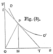
The illustration that accompanied Marshall's original definition of elasticity, the ratio of PT to Pt

Together with the concept of an economic "elasticity" coefficient, Alfred Marshall is credited with defining "elasticity of demand" in Principles of Economics, published in 1890.^[23] Alfred Marshall invented cost elasticity of need but four years later he had invented the concept of elasticity. He used Cournot'southward bones creating of the demand bend to become the equation for price elasticity of need. He described toll elasticity of demand as thus: "And we may say generally:— the elasticity (or responsiveness) of demand in a market is dandy or small according as the amount demanded increases much or fiddling for a given fall in cost, and diminishes much or fiddling for a given rising in cost".^[24] He reasons this since "the only universal constabulary as to a person's desire for a article is that information technology diminishes ... but this diminution may be tedious or rapid. If it is tiresome... a pocket-size autumn in price will cause a comparatively large increment in his purchases. Just if it is rapid, a pocket-size fall in toll will cause only a very small increase in his purchases. In the former instance... the elasticity of his wants, nosotros may say, is bully. In the latter case... the elasticity of his need is small."^[25] Mathematically, the Marshallian PED was based on a point-price definition, using differential calculus to calculate elasticities.^[26]

Determinants [edit]

The overriding factor in determining the elasticity is the willingness and ability of consumers later on a cost change to postpone immediate consumption decisions concerning the adept and to search for substitutes ("wait and look").^[27] A number of factors tin can thus affect the elasticity of demand for a good:^[28]

Availability of substitute goods

The more and closer the substitutes available, the college the elasticity is likely to be, as people can easily switch from 1 good to another if an even minor toll change is fabricated;^{[28] [29] [30]} In that location is a strong substitution result.^[31] If no close substitutes are available, the substitution effect will be small and the demand inelastic.^[31]

Breadth of definition of a good

The broader the definition of a good (or service), the lower the elasticity. For example, Company X'due south fish and chips would tend to have a relatively loftier elasticity of need if a significant number of substitutes are available, whereas food in full general would have an extremely low elasticity of demand because no substitutes be.^[32]

Percentage of income

The higher the percentage of the consumer'south income that the product'due south price represents, the higher the elasticity tends to be, as people will pay more attention when purchasing the proficient because of its toll;^{[28] [29]} The income issue is substantial.^[33] When the goods represent just a negligible portion of the budget the income upshot will be insignificant and demand inelastic,^[33]

Necessity

The more than necessary a expert is, the lower the elasticity, as people volition attempt to buy information technology no matter the cost, such equally the case of insulin for those who need it.^{[13] [29]}

Duration

For most goods, the longer a cost change holds, the higher the elasticity is likely to be, every bit more than and more consumers observe they have the fourth dimension and inclination to search for substitutes.^{[28] [30]} When fuel prices increase of a sudden, for instance, consumers may even so make full their empty tanks in the short run, merely when prices remain high over several years, more than consumers volition reduce their demand for fuel by switching to carpooling or public transportation, investing in vehicles with greater fuel economy or taking other measures.^[29] This does not hold for consumer durables such equally the cars themselves, however; eventually, it may get necessary for consumers to supersede their nowadays cars, so one would expect demand to be less rubberband.^[29]

Make loyalty

An zipper to a sure brand—either out of tradition or considering of proprietary barriers—tin override sensitivity to toll changes, resulting in more than inelastic demand.^{[32] [34]}

Who pays

Where the purchaser does not directly pay for the good they consume, such as with corporate expense accounts, need is likely to exist more inelastic.^[34]

Addictiveness

Goods that are more addictive in nature tend to take an inelastic PED (accented value of PED < 1). Examples of such include cigarettes, heroin and booze. This is because consumers view such appurtenances equally necessities and hence are forced to buy them, despite even significant price changes.

Relation to marginal revenue [edit]

The following equation holds:

${\displaystyle R'=P\,\left(i+{\dfrac {1}{E_{d}}}\right)}$

where

R′ is the marginal revenue

P is the price

Proof:

Define Full Revenue as R

${\displaystyle R'={\frac {\partial R}{\partial Q}}={\frac {\fractional }{\partial Q}}(P\,Q)=P+Q\,{\frac {\partial P}{\partial Q}}}$

${\displaystyle E_{d}={\dfrac {\partial Q}{\fractional P}}\cdot {\dfrac {P}{Q}}\Rightarrow E_{d}\cdot {\frac {Q}{P}}={\frac {\partial Q}{\partial P}}\Rightarrow {\frac {P}{E_{d}\cdot Q}}={\frac {\fractional P}{\partial Q}}}$

${\displaystyle R'=P+Q\cdot {\frac {P}{E_{d}\cdot Q}}=P\,\left(one+{\frac {1}{E_{d}}}\correct)}$

On a graph with both a need bend and a marginal acquirement curve, demand will be elastic at all quantities where marginal revenue is positive. Demand is unit of measurement elastic at the quantity where marginal acquirement is aught. Demand is inelastic at every quantity where marginal revenue is negative.^[35]

Issue on unabridged revenue [edit]

A set of graphs shows the relationship between demand and revenue (PQ) for the specific case of a linear demand curve. As price decreases in the elastic range, the revenue increases, but in the inelastic range, revenue falls. Revenue is highest at the quantity where the elasticity equals i.

A firm considering a price change must know what issue the change in cost will have on full revenue. Revenue is but the production of unit of measurement price times quantity:

${\displaystyle {\text{Revenue}}=PQ_{d}}$

Mostly, whatever change in toll will have ii effects:^[36]

The price outcome

For inelastic appurtenances, an increase in unit price will tend to increase revenue, while a decrease in price volition tend to decrease revenue. (The effect is reversed for rubberband goods.)

The quantity event

An increase in unit of measurement cost will tend to lead to fewer units sold, while a decrease in unit toll will tend to lead to more units sold.

For inelastic goods, considering of the inverse nature of the human relationship between price and quantity demanded (i.due east., the law of demand), the two effects touch total revenue in opposite directions. Just in determining whether to increment or decrease prices, a house needs to know what the internet result will exist. Elasticity provides the answer: The percentage alter in total revenue is approximately equal to the percentage modify in quantity demanded plus the percentage alter in price. (I change will be positive, the other negative.)^[37] The percentage change in quantity is related to the percentage change in toll by elasticity: hence the per centum alter in acquirement tin can be calculated past knowing the elasticity and the pct modify in price alone.

Equally a upshot, the relationship betwixt elasticity and revenue tin can be described for any good:^{[38] [39]}

• When the cost elasticity of demand for a skillful is perfectly inelastic (East _d = 0), changes in the price do not affect the quantity demanded for the skilful; raising prices will ever crusade total revenue to increase. Goods necessary to survival tin can be classified here; a rational person will be willing to pay annihilation for a practiced if the alternative is death. For example, a person in the desert weak and dying of thirst would easily give all the coin in his wallet, no matter how much, for a bottle of h2o if he would otherwise die. His demand is non contingent on the price.
• When the price elasticity of need is relatively inelastic (−1 < E _d < 0), the percentage change in quantity demanded is smaller than that in price. Hence, when the toll is raised, the total revenue increases, and vice versa.
• When the price elasticity of demand is unit (or unitary) elastic (E _d = −i), the percentage change in quantity demanded is equal to that in toll, so a change in price volition not touch total acquirement.
• When the price elasticity of demand is relatively elastic (−∞ < E _d < −1), the pct alter in quantity demanded is greater than that in toll. Hence, when the toll is raised, the total acquirement falls, and vice versa.
• When the price elasticity of demand is perfectly rubberband (E _d is − ∞), any increase in the price, no matter how small-scale, will cause the quantity demanded for the skillful to drop to zip. Hence, when the price is raised, the total acquirement falls to zero. This situation is typical for goods that have their value divers past police force (such equally fiat currency); if a five-dollar beak were sold for anything more v dollars, nobody would buy information technology, so need is nil (assuming that the neb does not accept a misprint or something else which would cause it to accept its ain inherent value).

Hence, as the accompanying diagram shows, full revenue is maximized at the combination of price and quantity demanded where the elasticity of demand is unitary.^[39]

Information technology is important to realize that price-elasticity of need is not necessarily constant over all price ranges. The linear demand curve in the accompanying diagram illustrates that changes in price besides change the elasticity: the toll elasticity is different at every point on the curve.

Effect on tax incidence [edit]

When demand is more than inelastic than supply, consumers will bear a greater proportion of the tax burden than producers will.

Need elasticity, in combination with the cost elasticity of supply can be used to appraise where the incidence (or "burden") of a per-unit tax is falling or to predict where information technology will fall if the tax is imposed. For example, when demand is perfectly inelastic, past definition consumers have no alternative to purchasing the adept or service if the price increases, so the quantity demanded would remain abiding. Hence, suppliers can increase the price by the full amount of the tax, and the consumer would end upward paying the entirety. In the opposite case, when demand is perfectly elastic, by definition consumers have an infinite power to switch to alternatives if the price increases, then they would finish ownership the expert or service in question completely—quantity demanded would fall to goose egg. As a result, firms cannot pass on whatsoever role of the revenue enhancement by raising prices, and then they would exist forced to pay all of information technology themselves.^[40]

In practice, demand is likely to exist only relatively elastic or relatively inelastic, that is, somewhere between the extreme cases of perfect elasticity or inelasticity. More generally, then, the higher the elasticity of demand compared to Foot, the heavier the burden on producers; conversely, the more inelastic the demand compared to supply, the heavier the burden on consumers. The general principle is that the party (i.e., consumers or producers) that has fewer opportunities to avert the taxation by switching to alternatives will behave the greater proportion of the taxation brunt.^[forty] In the end the whole tax brunt is carried by individual households since they are the ultimate owners of the means of production that the firm utilises (encounter Circular menses of income).

PED and PES can also have an consequence on the deadweight loss associated with a tax regime. When PED, Human foot or both are inelastic, the deadweight loss is lower than a comparable scenario with higher elasticity.

Optimal pricing [edit]

Amongst the most common applications of price elasticity is to determine prices that maximize acquirement or turn a profit.

Abiding elasticity and optimal pricing [edit]

If one point elasticity is used to model need changes over a finite range of prices, elasticity is implicitly assumed constant with respect to price over the finite price range. The equation defining price elasticity for one product can be rewritten (omitting secondary variables) equally a linear equation.

${\displaystyle LQ=1000+E\times LP}$

where

${\displaystyle LQ=\ln(Q),LP=\ln(P),E}$ is the elasticity, and ${\displaystyle K}$ is a constant.

Similarly, the equations for cross elasticity for ${\displaystyle due north}$ products tin can be written as a fix of ${\displaystyle n}$ simultaneous linear equations.

${\displaystyle LQ_{l}=K_{l}+E_{50,thou}\times LP^{grand}}$

where

${\displaystyle l}$ and ${\displaystyle thousand=1,\dotsc ,northward,LQ_{l}=\ln(Q_{l}),LP^{fifty}=\ln(P^{l})}$ , and ${\displaystyle K_{l}}$ are constants; and appearance of a letter index as both an upper index and a lower alphabetize in the same term implies summation over that alphabetize.

This form of the equations shows that point elasticities assumed constant over a price range cannot determine what prices generate maximum values of ${\displaystyle \ln(Q)}$ ; similarly they cannot predict prices that generate maximum ${\displaystyle Q}$ or maximum revenue.

Constant elasticities can predict optimal pricing but past computing point elasticities at several points, to determine the toll at which betoken elasticity equals −ane (or, for multiple products, the set of prices at which the point elasticity matrix is the negative identity matrix).

Non-constant elasticity and optimal pricing [edit]

If the definition of price elasticity is extended to yield a quadratic relationship between demand units ( ${\displaystyle Q}$ ) and price, then it is possible to compute prices that maximize ${\displaystyle \ln(Q)}$ , ${\displaystyle Q}$ , and revenue. The cardinal equation for 1 production becomes

${\displaystyle LQ=M+E_{1}\times LP+E_{ii}\times LP^{2}}$

and the corresponding equation for several products becomes

${\displaystyle LQ_{l}=K_{l}+E1_{l,g}\times LP^{k}+E2_{l,one thousand}\times (LP^{one thousand})^{2}}$

Excel models are available that compute constant elasticity, and utilise non-abiding elasticity to estimate prices that optimize revenue or turn a profit for 1 production^[41] or several products.^[42]

Limitations of revenue-maximizing strategies [edit]

In most situations, such as those with nonzero variable costs, revenue-maximizing prices are not profit-maximizing prices. For these situations, using a technique for Profit maximization is more appropriate.

Selected toll elasticities [edit]

Various enquiry methods are used to calculate the price elasticities in real life, including analysis of historic sales data, both public and individual, and use of present-solar day surveys of customers' preferences to build up test markets capable of modelling such changes.^[43] Alternatively, conjoint analysis (a ranking of users' preferences which can then exist statistically analysed) may exist used.^[44] Estimate estimates of price elasticity can be calculated from the income elasticity of need, under conditions of preference independence. This approach has been empirically validated using bundles of goods (east.m. nutrient, healthcare, education, recreation, etc.).^[45]

Though elasticities for nearly demand schedules vary depending on price, they tin can be modeled assuming abiding elasticity.^[46] Using this method, the elasticities for diverse appurtenances—intended to human activity as examples of the theory described higher up—are as follows. For suggestions on why these goods and services may have the elasticity shown, come across the above section on determinants of cost elasticity.

Cigarettes (Us)[47] −0.3 to −0.six (General) −0.6 to −0.seven (Youth) Alcoholic beverages (US)[48] −0.3 or −0.vii to −0.nine as of 1972 (Beer) −ane.0 (Wine) −1.5 (Spirits) Airline travel (US)[49] −0.3 (Start Class) −0.9 (Disbelieve) −1.5 (for Pleasure Travelers) Livestock −0.5 to −0.half dozen (Broiler Chickens)[50] Oil (World) −0.4 Car fuel[51] −0.09 (Short run) −0.31 (Long run) −0.085 to −0.thirteen (not-linear with price modify in the curt-run for Saudi Arabia in 2013[52]) Medicine (US) −0.31 (Medical insurance)[53] −0.03 to −0.06 (Pediatric Visits)[54] Patents −0.30 to −0.l[55]

Rice[56] −0.47 (Republic of austria) −0.viii0 (Bangladesh) −0.eight0 (Mainland china) −0.25 (Japan) −0.55 (US) Cinema visits (Us) −0.87 (General)[53] Alive Performing Arts (Theater, etc.) −0.iv to −0.ix[57] Transport −0.20 (Coach travel US)[53] −ii.80 (Ford meaty automobile)[58] −0.52 (Commuter parking)[59] Cannabis (US)[60] −0.655 Soft drinks −0.8 to −1.0 (general)[61] −iii.8 (Coca-Cola)[62] −iv.4 (Mountain Dew)[62] Steel −0.ii to −0.3[63] Telecommunications −0.405 (Mobile)[64] −0.434 (Broadband)[65] Eggs −0.one (US: Household simply)[66] −0.35 (Canada)[67] −0.55 (South Africa)[68] Golf game −0.3 to −0.7[63] University education near 0[69]

See as well [edit]

• Arc elasticity
• Cross elasticity of demand
• Income elasticity of demand
• Price elasticity of supply
• Supply and demand

Notes [edit]

1. ^ "Price elasticity of demand | Economics Online". 2020-01-fourteen. Retrieved 2021-04-xiv .
2. ^ Browning, Edgar K. (1992). Microeconomic theory and applications. New York City: HarperCollins. pp. 94–95. ISBN9780673521422.
3. ^ ^{a b} Png, Ivan (1989). p. 57.
4. ^ Parkin; Powell; Matthews (2002). pp. 74–five.
5. ^ ^{a b} Gillespie, Andrew (2007). p. 43.
6. ^ ^{a b} Gwartney, Yaw Bugyei-Kyei.James D.; Stroup, Richard 50.; Sobel, Russell Due south. (2008). p. 425.
7. ^ Gillespie, Andrew (2007). p. 57.
8. ^ Ruffin; Gregory (1988). p. 524.
9. ^ Ferguson, C.E. (1972). p. 106.
10. ^ Ruffin; Gregory (1988). p. 520
11. ^ McConnell; Brue (1990). p. 436.
12. ^ Economics, Tenth edition, John Sloman
13. ^ ^{a b} Parkin; Powell; Matthews (2002). p .75.
14. ^ McConnell; Brue (1990). p. 437
15. ^ ^{a b} Ruffin; Gregory (1988). pp. 518–519.
16. ^ ^{a b} Ferguson, C.E. (1972). pp. 100–101.
17. ^ ^{a b} Wall, Stuart; Griffiths, Alan (2008). pp. 53–54.
18. ^ ^{a b} McConnell;Brue (1990). pp. 434–435.
19. ^ Ferguson, C.E. (1972). p. 101n.
20. ^ Sloman, John (2006). p. 55.
21. ^ Wessels, Walter J. (2000). p. 296.
22. ^ Mas-Colell; Winston; Green (1995).
23. ^ Taylor, John (2006). p. 93.
24. ^ Marshall, Alfred (1890). III.IV.2.
25. ^ Marshall, Alfred (1890). 3.IV.i.
26. ^ Schumpeter, Joseph Alois; Schumpeter, Elizabeth Boody (1994). p. 959.
27. ^ Negbennebor (2001).
28. ^ ^{a b c d} Parkin; Powell; Matthews (2002). pp. 77–9.
29. ^ ^{a b c d e} Walbert, Mark. "Tutorial 4a". Retrieved 27 February 2010.
30. ^ ^{a b} Goodwin, Nelson, Ackerman, & Weisskopf (2009).
31. ^ ^{a b} Frank (2008) 118.
32. ^ ^{a b} Gillespie, Andrew (2007). p. 48.
33. ^ ^{a b} Frank (2008) 119.
34. ^ ^{a b} Png, Ivan (1999). pp. 62–three.
35. ^ Reed, Jacob (2016-05-26). "AP Microeconomics Review: Elasticity Coefficients". APEconReview.com . Retrieved 2016-05-27 .
36. ^ Krugman, Wells (2009). p. 151.
37. ^ Goodwin, Nelson, Ackerman & Weisskopf (2009). p. 122.
38. ^ Gillespie, Andrew (2002). p. 51.
39. ^ ^{a b} Arnold, Roger (2008). p. 385.
40. ^ ^{a b} Wall, Stuart; Griffiths, Alan (2008). pp. 57–58.
41. ^ "Pricing Tests and Cost Elasticity for i product". Archived from the original on 2012-11-13. Retrieved 2013-03-03 .
42. ^ "Pricing Tests and Price Elasticity for several products". Archived from the original on 2012-11-13. Retrieved 2013-03-03 .
43. ^ Samia Rekhi (16 May 2016). "Empirical Estimation of Demand: Top 10 Techniques". economicsdiscussion.net . Retrieved 11 December 2020.
44. ^ Png, Ivan (1999). pp. 79–fourscore.
45. ^ Sabatelli, Lorenzo (2016-03-21). "Human relationship between the Uncompensated Price Elasticity and the Income Elasticity of Demand under Conditions of Condiment Preferences". PLOS ONE. 11 (3): e0151390. arXiv:1602.08644. Bibcode:2016PLoSO..1151390S. doi:ten.1371/journal.pone.0151390. ISSN 1932-6203. PMC4801373. PMID 26999511.
46. ^ "Constant Elasticity Demand and Supply Curves (Q=A*P^c)". Archived from the original on 13 January 2011. Retrieved 26 Apr 2010.
47. ^ Perloff, J. (2008). p. 97.
48. ^ Chaloupka, Frank J.; Grossman, Michael; Saffer, Henry (2002); Hogarty and Elzinga (1972) cited past Douglas (1993).
49. ^ Pindyck; Rubinfeld (2001). p. 381.; Steven Morrison in Duetsch (1993), p. 231.
50. ^ Richard T. Rogers in Duetsch (1993), p. 6.
51. ^ Havranek, Tomas; Irsova, Zuzana; Janda, Karel (2012). "Need for gasoline is more price-inelastic than normally thought" (PDF). Energy Economics. 34: 201–207. doi:10.1016/j.eneco.2011.09.003.
52. ^ Algunaibet, Ibrahim; Matar, Walid (2018). "The responsiveness of fuel demand to gasoline price change in passenger send: a instance study of Saudi arabia". Energy Efficiency. 11 (half dozen): 1341–1358. doi:10.1007/s12053-018-9628-half-dozen. S2CID 157328882.
53. ^ ^{a b c} Samuelson; Nordhaus (2001).
54. ^ Goldman and Grossman (1978) cited in Feldstein (1999), p. 99
55. ^ de Rassenfosse and van Pottelsberghe (2007, pp. 598; 2012, p. 72)
56. ^ Perloff, J. (2008).
57. ^ Heilbrun and Gray (1993, p. 94) cited in Vogel (2001)
58. ^ Goodwin; Nelson; Ackerman; Weisskopf (2009). p. 124.
59. ^ Lehner, S.; Peer, S. (2019), The toll elasticity of parking: A meta-analysis, Transportation Research Function A: Policy and Practice, Volume 121, March 2019, pages 177−191" web|url=https://doi.org/x.1016/j.tra.2019.01.014
60. ^ Davis, A.; Nichols, K. (2013), The Price Elasticity of Marijuana Demand"
61. ^ Brownell, Kelly D.; Farley, Thomas; Willett, Walter C. et al. (2009).
62. ^ ^{a b} Ayers; Collinge (2003). p. 120.
63. ^ ^{a b} Barnett and Crandall in Duetsch (1993), p. 147
64. ^ "Valuing the Outcome of Regulation on New Services in Telecommunication" (PDF). Jerry A. Hausman. Retrieved 29 September 2016.
65. ^ "Price and Income Elasticity of Demand for Broadband Subscriptions: A Cross-Exclusive Model of OECD Countries" (PDF). SPC Network. Retrieved 29 September 2016.
66. ^ Krugman and Wells (2009) p. 147.
67. ^ "Profile of The Canadian Egg Manufacture". Agronomics and Agri-Food Canada. Archived from the original on viii July 2011. Retrieved ix September 2010.
68. ^ Cleasby, R. C. Grand.; Ortmann, G. F. (1991). "Demand Analysis of Eggs in South Africa". Agrekon. 30 (ane): 34–36. doi:10.1080/03031853.1991.9524200.
69. ^ Havranek, Tomas; Irsova, Zuzana; Zeynalova, Olesia (2018). "Tuition Fees and University Enrolment: A Meta‐Regression Analysis". Oxford Bulletin of Economics and Statistics. 80 (6): 1145–1184. doi:10.1111/obes.12240. S2CID 158193395.

References [edit]

• Arnold, Roger A. (17 December 2008). Economics. Cengage Learning. ISBN978-0-324-59542-0 . Retrieved 28 February 2010.
• Ayers; Collinge (2003). Microeconomics. Pearson. ISBN978-0-536-53313-v.
• Brownell, Kelly D.; Farley, Thomas; Willett, Walter C.; Popkin, Barry M.; Chaloupka, Frank J.; Thompson, Joseph Westward.; Ludwig, David S. (fifteen October 2009). "The Public Wellness and Economical Benefits of Taxing Sugar-Sweetened Beverages". New England Journal of Medicine. 361 (16): 1599–1605. doi:10.1056/NEJMhpr0905723. PMC3140416. PMID 19759377.
• Browning, Edgar K.; Browning, Jacquelene M. (1992). Microeconomic Theory and Applications (4th ed.). HarperCollins. Retrieved xi December 2020.
• Case, Karl; Fair, Ray (1999). Principles of Economics (fifth ed.). Prentice-Hall. ISBN978-0-13-961905-2.
• Chaloupka, Frank J.; Grossman, Michael; Saffer, Henry (2002). "The effects of toll on alcohol consumption and alcohol-related problems". Alcohol Research and Health. 26 (1): 22–34. PMC6683806. PMID 12154648.
• de Rassenfosse, Gaetan; van Pottelsberghe, Bruno (2007). "Per united nations pugno di dollari: a first expect at the price elasticity of patents". Oxford Review of Economic Policy. 23 (iv): 588–604. doi:10.1093/oxrep/grm032. S2CID 55387166. Working paper on RePEc
• de Rassenfosse, Gaetan; van Pottelsberghe, Bruno (2012). "On the price elasticity of demand for patents". Oxford Message of Economics and Statistics. 74 (1): 58–77. doi:10.1111/j.1468-0084.2011.00638.x. S2CID 43660064. Working paper on RePEc
• Duetsch, Larry Fifty. (1993). Industry Studies. Englewood Cliffs, NJ: Prentice Hall. ISBN978-0-585-01979-6.
• Feldstein, Paul J. (1999). Wellness Care Economics (5th ed.). Albany, NY: Delmar Publishers. ISBN978-0-7668-0699-3.
• Ferguson, Charles Due east. (1972). Microeconomic Theory (3rd ed.). Homewood, Illinois: Richard D. Irwin. ISBN978-0-256-02157-8.
• Frank, Robert (2008). Microeconomics and Behavior (7th ed.). McGraw-Hill. ISBN978-0-07-126349-8.
• Gillespie, Andrew (1 March 2007). Foundations of Economics. Oxford University Press. ISBN978-0-19-929637-8 . Retrieved 28 February 2010.
• Goodwin; Nelson; Ackerman; Weisskopf (2009). Microeconomics in Context (2nd ed.). Sharpe. ISBN978-0-618-34599-1.
• Gwartney, James D.; Stroup, Richard L.; Sobel, Russell S.; David MacPherson (14 Jan 2008). Economic science: Individual and Public Choice. Cengage Learning. ISBN978-0-324-58018-ane . Retrieved 28 February 2010.
• Krugman; Wells (2009). Microeconomics (2d ed.). Worth. ISBN978-0-7167-7159-iii.
• Landers (February 2008). Estimates of the Price Elasticity of Need for Casino Gaming and the Potential Furnishings of Casino Tax Hikes.
• Marshall, Alfred (1920). Principles of Economics. Library of Economic science and Freedom. ISBN978-0-256-01547-8 . Retrieved 5 March 2010.
• Mas-Colell, Andreu; Winston, Michael D.; Greenish, Jerry R. (1995). Microeconomic Theory. New York: Oxford University Press. ISBN978-1-4288-7151-9.
• McConnell, Campbell R.; Brue, Stanley L. (1990). Economic science: Principles, Bug, and Policies (11th ed.). New York: McGraw-Hill. ISBN978-0-07-044967-1.
• Negbennebor (2001). "The Freedom to Cull". Microeconomics. ISBN978-i-56226-485-7.
• Parkin, Michael; Powell, Melanie; Matthews, Kent (2002). Economics. Harlow: Addison-Wesley. ISBN978-0-273-65813-9.
• Perloff, J. (2008). Microeconomic Theory & Applications with Calculus. Pearson. ISBN978-0-321-27794-7.
• Pindyck; Rubinfeld (2001). Microeconomics (fifth ed.). Prentice-Hall. ISBN978-1-4058-9340-4.
• Png, Ivan (1999). Managerial Economics. Blackwell. ISBN978-0-631-22516-4 . Retrieved 28 February 2010.
• Ruffin, Roy J.; Gregory, Paul R. (1988). Principles of Economics (3rd ed.). Glenview, Illinois: Scott, Foresman. ISBN978-0-673-18871-7.
• Samuelson; Nordhaus (2001). Microeconomics (17th ed.). McGraw-Hill. ISBN978-0-07-057953-8.
• Schumpeter, Joseph Alois; Schumpeter, Elizabeth Boody (1994). History of economical analysis (12th ed.). Routledge. ISBN978-0-415-10888-1 . Retrieved 5 March 2010.
• Sloman, John (2006). Economics. Financial Times Prentice Hall. ISBN978-0-273-70512-3 . Retrieved 5 March 2010.
• Taylor, John B. (1 February 2006). Economics. Cengage Learning. ISBN978-0-618-64085-0 . Retrieved 5 March 2010.
• Vogel, Harold (2001). Entertainment Manufacture Economics (5th ed.). Cambridge University Press. ISBN978-0-521-79264-6.
• Wall, Stuart; Griffiths, Alan (2008). Economics for Business and Management. Fiscal Times Prentice Hall. ISBN978-0-273-71367-8 . Retrieved 6 March 2010.
• Wessels, Walter J. (ane September 2000). Economics. Barron'southward Educational Series. ISBN978-0-7641-1274-4 . Retrieved 28 February 2010.

External links [edit]

• A Lesson on Elasticity in Four Parts, Youtube, Jodi Beggs
• Price Elasticity Models and Optimization
• Approx. PED of Various Products (U.Southward.)
• Approx. PED of Various Domicile-Consumed Foods (U.Thousand.)

andersonevestan43.blogspot.com

Source: https://en.wikipedia.org/wiki/Price_elasticity_of_demand

Share this post